Benchmarking against a plain R approach • mdl

A critical reader might suggest that, given that mdl::mtrx() does quite a bit less than model.matrix(), it’s not really suprising that it would run more quickly than model.matrix(). How fast could we make an analogue to mdl::mtrx() in “plain R” (i.e. without rust)? Let’s see.

library(mdl)
library(bench)
library(ggplot2)
library(dplyr)

A plain R alternative

mdl::mtrx() is mostly just a glorified as.matrix() method for data frames that makes dummy variables out of factors, characters, and logicals. Let’s see if we mock up a plain R alternative, mdl_mtrx(), that’s just as fast.

First, we’ll write a helper to apply to factors to convert them to dummy variables, loosely based on hardhat::fct_encode_one_hot().

x <- factor(sample(letters[1:3], 100, replace = TRUE))

fct_encode_dummy <- function(x) {
  row_names <- names(x)
  col_names <- levels(x)
  col_names <- col_names[-1]
  dim_names <- list(row_names, col_names)
  n_cols <- length(col_names)
  n_rows <- length(x)
  x <- unclass(x)
  out <- matrix(0L, nrow = n_rows, ncol = n_cols, dimnames = dim_names)
  loc <- cbind(row = seq_len(n_rows), col = x - 1)
  out[loc] <- 1L
  out
}

It’s hard to beat R at converting characters to factors, so we’ll convert character vectors to factors and then to dummy variables via fct_encode_dummy(). The rest of the variable types we’ll test here are one-liners.

to_numeric <- function(x) {
  switch(
    class(x),
    numeric = x,
    integer = x,
    character = fct_encode_dummy(as.factor(x)),
    factor = fct_encode_dummy(x),
    logical = x
  )
}
  
mdl_mtrx <- function(formula, data) {
  predictors <- mdl:::predictors(formula, data)
  
  cols <- lapply(data[predictors], to_numeric)
  do.call(cbind, cols)
}

We’ll use a data frame with a variety of types to benchmark in this article. Wrapping in a quick function:

create_data_frame <- function(n_rows) {
  data.frame(
    outcome = runif(n_rows),
    pred_numeric = runif(n_rows),
    pred_integer = sample(c(0L, 1L), n_rows, replace = TRUE),
    pred_logical = sample(c(TRUE, FALSE), n_rows, replace = TRUE),
    pred_factor_2 = factor(sample(letters[1:2], n_rows, replace = TRUE)),
    pred_factor_3 = factor(sample(letters[1:3], n_rows, replace = TRUE)),
    pred_character_2 = sample(letters[1:2], n_rows, replace = TRUE),
    pred_character_3 = sample(letters[1:3], n_rows, replace = TRUE)
  )
}

d <- create_data_frame(5)

d
#>     outcome pred_numeric pred_integer pred_logical pred_factor_2 pred_factor_3
#> 1 0.2485387    0.1645692            0         TRUE             a             a
#> 2 0.4028812    0.6632066            0         TRUE             b             b
#> 3 0.7696302    0.8565750            1         TRUE             a             b
#> 4 0.1194854    0.9265464            0         TRUE             b             c
#> 5 0.1946950    0.5523776            0        FALSE             b             c
#>   pred_character_2 pred_character_3
#> 1                b                c
#> 2                a                a
#> 3                b                a
#> 4                b                c
#> 5                a                c

Passing each of those data types to make sure our new function mdl_mtrx() does what we want in the simplest case:

mdl_mtrx(outcome ~ ., d)
#>      pred_numeric pred_integer pred_logical b b c b c
#> [1,]    0.1645692            0            1 0 0 0 1 1
#> [2,]    0.6632066            0            1 1 1 0 0 0
#> [3,]    0.8565750            1            1 0 1 0 1 0
#> [4,]    0.9265464            0            1 1 0 1 1 1
#> [5,]    0.5523776            0            0 1 0 1 0 1

Okay, so, no type checking, plenty of issues with edge cases, lean and mean R function. Let’s check the timings out, first on a very small dataset:

d <- create_data_frame(30)

bench::mark(
  mdl_mtrx = mdl_mtrx(outcome ~ ., d),
  `mdl::mtrx` = mdl::mtrx(outcome ~ ., d),
  model.matrix = model.matrix(outcome ~ ., d),
  check = FALSE
)
#> # A tibble: 3 × 6
#>   expression        min   median `itr/sec` mem_alloc `gc/sec`
#>   <bch:expr>   <bch:tm> <bch:tm>     <dbl> <bch:byt>    <dbl>
#> 1 mdl_mtrx        156µs    167µs     5888.      38KB     21.9
#> 2 mdl::mtrx       198µs    211µs     4604.     801KB     19.0
#> 3 model.matrix    780µs    831µs     1198.     488KB     23.8

Not bad, scrappy little feller! Now, on a few more reasonably sized datasets:

res <- 
  bench::press(
    n_rows = 10^seq(2:8), 
    {
      d <- create_data_frame(n_rows)
      bench::mark(
        mdl_mtrx = mdl_mtrx(outcome ~ ., d),
        `mdl::mtrx` = mdl::mtrx(outcome ~ ., d),
        model.matrix = model.matrix(outcome ~ ., d),
        check = FALSE
      )
    }
  )

ggplot(res) +
  aes(x = n_rows, y = median, col = expression) +
  geom_point() +
  scale_x_log10()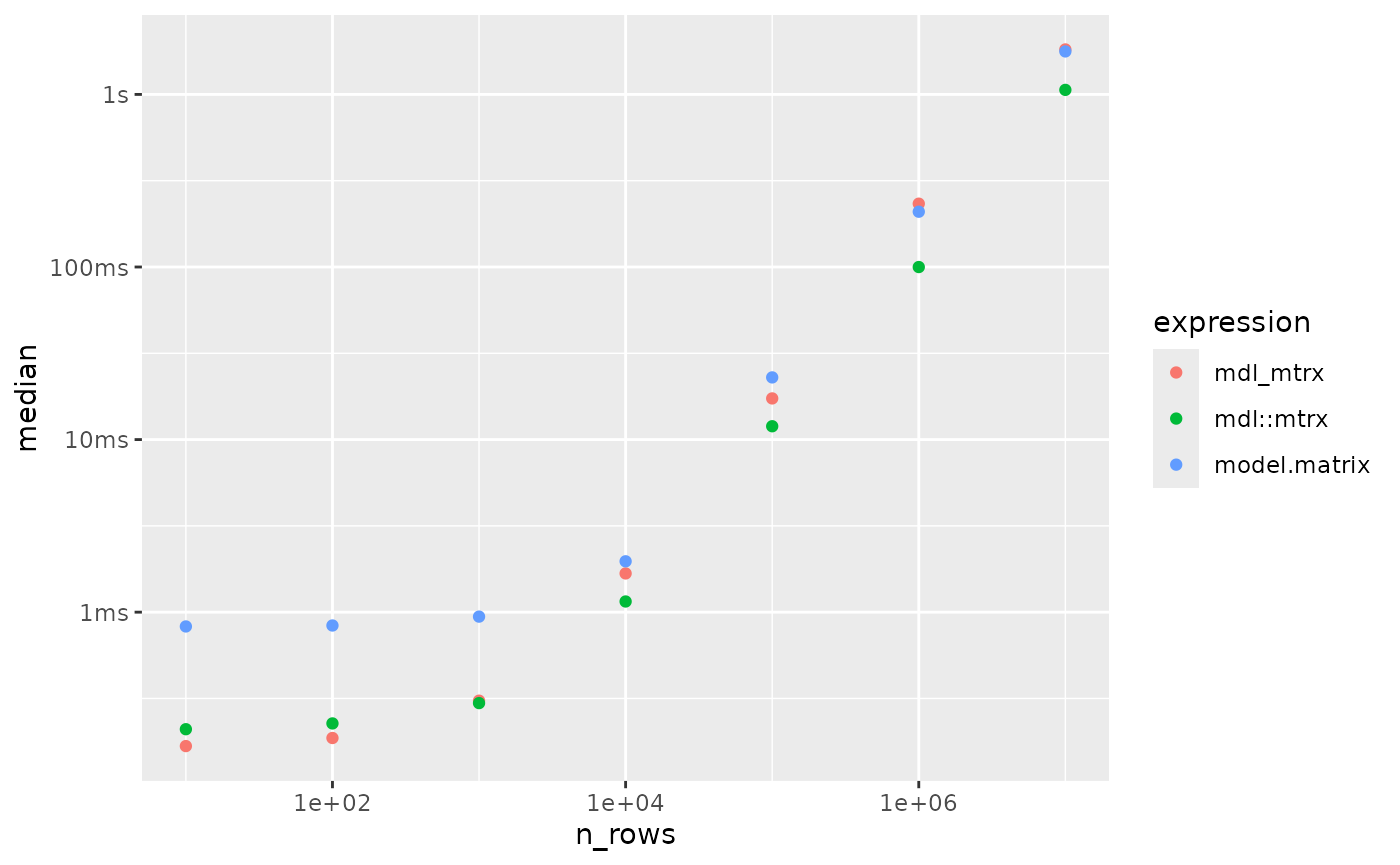

If the log scale is tripping you up, here’s a slice of data for the largest numbers of rows:

res %>% 
  select(expression, median, mem_alloc) %>%
  tail(3)
#> # A tibble: 3 × 3
#>   expression     median mem_alloc
#>   <bch:expr>   <bch:tm> <bch:byt>
#> 1 mdl_mtrx        1.82s    3.02GB
#> 2 mdl::mtrx       1.06s    1.84GB
#> 3 model.matrix    1.77s    4.06GB

timings <- res %>% 
  tail(3) %>%
  pull(median) %>%
  as.numeric()

In this timing, model.matrix() took 1.7x slower than mdl::mtrx(), and our speedy plain R approach took 1.7x as long.